This is the multi-page printable view of this section. .
pgvecto.rs Documentation
-
1: Getting Started
- 1.1: Overview
- 1.2: Installation
-
2: Usage
- 2.1: Indexing
- 2.2: Search
- 2.3: Monitoring
- 2.4: Quantization
- 2.5: `pgvector` compatibility
-
3: Use Cases
- 3.1: Hybrid Search
- 3.2: Adaptive retrieval and shortening embeddings
- 3.3: Image Search
- 3.4: Multi Tenancy
- 3.5: Sparse Vector Search
- 3.6: Generative Question-Answering
-
4: Integration
- 4.1: LangChain
- 4.2: LlamaIndex
- 4.3: Citus
-
5: Administration
- 5.1: Configuration
- 5.2: Upgrading
- 5.3: Logical replication
- 5.4: Foreign data wrapper (FDW)
- 5.5: Kubernetes
- 5.6: Migration
-
6: FAQs
- 6.1: General FAQ
- 6.2: Comparison with pgvector
- 6.3: Why not a specialty vector database?
- 6.4: Benchmarks
-
7: Reference
- 7.1: Schema
- 7.2: Indexing Options
- 7.3: Search Options
-
7.4: Vector Types
- 7.4.1: Half-Precision Vector: `vecf16`
- 7.4.2: 8-Bit Integer Vector: `veci8`
- 7.4.3: Sparse Vector: `svector`
- 7.4.4: Binary Vector: `bvector`
-
8: Community
- 8.1: Contributing to `pgvecto.rs`
- 8.2: Roadmap
- 8.3: Adopters
-
9: Developers
- 9.1: Development
pgvecto.rs has been succeeded by vchord. For new deployments, use vchord; for existing pgvecto.rs databases, follow the Migration Guide.
1 - Getting Started
1.1 - Overview
We strongly suggest you explore our new VectorChord implementation, offering enhanced stability and performance. Users are advised to transition to VectorChord. Refer to the migration guide for assistance.
An introduction to the pgvecto.rs.
What is pgvecto.rs
pgvecto.rs is a Postgres extension that provides vector similarity search functions. It is written in Rust and based on pgrx. It is currently in the beta status, we invite you to try it out in production and provide us with feedback. Read more at 📝our launch blog.
Comparison with pgvector
Checkout pgvecto.rs vs pgvector for more details.
| Feature | pgvecto.rs | pgvector |
|---|---|---|
| Filtering | Introduces VBASE method for vector search and relational query (e.g. Single-Vector TopK + Filter + Join). | When filters are applied, the results may be incomplete. For example, if you originally intended to limit the results to 10, you might end up with only 5 results with filters. |
| Vector Dimensions | Supports up to 65535 dimensions. | Supports up to 2000 dimensions. |
| SIMD | SIMD instructions are dynamically dispatched at runtime to maximize performance based on the capabilities of the specific machine. | Added CPU dispatching for distance functions on Linux x86-64" in 0.7.0. |
| Data Types | Introduces additional data types: binary vectors, FP16 (16-bit floating point), and INT8 (8-bit integer). | - |
| Indexing | Handles the storage and memory of indexes separately from PostgreSQL | Relies on the native storage engine of PostgreSQL |
| WAL Support | Provides Write-Ahead Logging (WAL) support for data, index support is working in progress. | Provides Write-Ahead Logging (WAL) support for index and data. |
Quick start
For new users, we recommend using the Docker image to get started quickly.
Then you can connect to the database using the psql command line tool. The default username is postgres, and the default password is mysecretpassword.
Run the following SQL to ensure the extension is enabled.
pgvecto.rs introduces a new data type vector(n) denoting an n-dimensional vector. The n within the brackets signifies the dimensions of the vector.
You could create a table with the following SQL.
vector(n) is a valid data type only if . Due to limits of PostgreSQL, it’s possible to create a value of type vector(3) of dimensions and vector is also a valid data type. However, you cannot still put scalar or more than scalars to a vector. If you use vector for a column or there is some values mismatched with dimension denoted by the column, you won’t able to create an index on it.
You can then populate the table with vector data as follows.
We support three operators to calculate the distance between two vectors.
<->: squared Euclidean distance, defined as .<#>: negative dot product, defined as .<=>: cosine distance, defined as .
You can search for a vector simply like this.
A simple Question-Answering application
Please check out the Question-Answering application tutorial.
Half-precision floating-point
vecf16 type is the same with vector in anything but the scalar type. It stores 16-bit floating point numbers. If you want to reduce the memory usage to get better performance, you can try to replace vector type with vecf16 type.
For more usage of vecf16, please refer to vector types.
Sparse vector
svector type is a sparse vector type. It stores a vector in a sparse format. It is suitable for vectors with many zeros.
For more usage of svector, please refer to vector types.
Binary vector
bvector type is a binary vector type. It is a fixed-length bit string. Except for above 3 distances, we also support jaccard distance <~>, which defined as . And hamming distance is the same with squared Euclidean distance, you can use <-> operator to calculate it. We also provide binarize function to construct a bvector from a vector, which set the positive elements to 1, otherwise 0.
For more usage of bvector, please refer to vector types.
Roadmap 🗂️
Please check out ROADMAP.
Contribute 😊
We welcome all kinds of contributions from the open-source community, individuals, and partners.
- Join our discord community!
- To build from the source, please read our contributing documentation and development tutorial.
Talk with us
💬 Interested in talking with us about your experience building or managing AI/ML applications?
1.2 - Installation
We strongly encourage you to explore our new VectorChord implementation, which offers improved stability and performance. Users are encouraged to migrate to VectorChord. See the migration guide for assistance.
There are four ways to install pgvecto.rs.
Docker

The easiest way to try pgvecto.rs is to run it from a ready-to use Docker image.
Then you can connect to the database using the psql command line tool. The default username is postgres, and the default password is mysecretpassword.
Run the following SQL to ensure the extension is enabled.
To achieve full performance, please mount the volume to pg data directory by adding the option like -v $PWD/pgdata:/var/lib/postgresql/data
You can configure PostgreSQL by the reference of the parent image in https://hub.docker.com/_/postgres/.
From Debian package
Installation from the Debian package requires a dependency on GLIBC >= 2.31, e.g:
Ubuntu 20.04or laterDebian Bullseyeor later
Debian packages(.deb) are used in distributions based on Debian, such as Ubuntu and many others. They can be easily installed by dpkg or apt-get.
-
Download the deb package in the release page, and type
sudo apt install vectors-pg15-*.debto install the deb package. -
Configure your PostgreSQL by modifying the
shared_preload_librariesandsearch_pathto include the extension.
- Connect to the database and enable the extension.
From ZIP package
since v0.2.1Installation from the ZIP package requires a dependency on GLIBC >= 2.31, e.g:
RHEL 9or later
For systems that are not Debian based and cannot run a Docker container, please follow these steps to install:
- Before install, make sure that you have the necessary packages installed, including
PostgreSQL,pg_config,unzip,wget.
- Verify whether
$pkglibdirand$shardirhave been set by PostgreSQL.
- Download the zip package in the release page and extract it to a temporary directory.
- Copy the extension files to the PostgreSQL directory.
- Configure your PostgreSQL by modifying the
shared_preload_librariesandsearch_pathto include the extension.
- Connect to the database and enable the extension.
From source
Before building from source, you could refer to the development guide to set up the development environment.
- Then you could build and install the extension.
- Configure your PostgreSQL by modifying the
shared_preload_librariesandsearch_pathto include the extension.
- Connect to the database and enable the extension.
2 - Usage
2.1 - Indexing
Indexing is the process of building a data structure that allows for efficient search. pgvecto.rs supports three indexing algorithms: brute force (flat), IVF, and HNSW. The default algorithm is HNSW.
To construct an index for vectors, first create a table named items with a column named embedding of type vector(n). Then, populate the table with generated data.
vector is the suitable data type for most situations. pgvecto.rs also supports other specific vector types, including:
- Half-Precision Vector
- 8-Bit Integer Vector since v0.3.0
- Sparse Vector since v0.3.0
- Binary Vector since v0.3.0
You can create a vector index for squared Euclidean distance with the following SQL.
The vector_l2_ops operator class calculates squared Euclidean distance. Refer to the documentation for a list of operator classes.
To switch the indexing algorithm from the default HNSW to IVF, execute the SQL command below. For additional examples of usage, refer to the documentation.
You can now perform a KNN search with the following SQL, leveraging the vector index for your query.
pgvecto.rs constructs the index asynchronously. When you insert new rows into the table, they will first be placed in an append-only file. The background thread will periodically merge the newly inserted row to the existing index. When a user performs any search prior to the merge process, it scans the append-only file to ensure accuracy and consistency.
Examples
Here are some examples of how to create indexes using various algorithms and settings. For a complete list of options, please consult the reference guide.
Suggestions
Selecting the appropriate indexing algorithm and settings is crucial for vector search performance. Below are recommendations tailored to various use cases.
Brute force (flat)
If you’re conducting a limited number of searches (between 1,000 and 10,000) or require precise results, the brute force algorithm is a viable option.
This algorithm sets the standard for other indexing methods. It retains vectors in their original form without compression and avoids additional overhead. While straightforward and user-friendly, it’s not ideal for processing large datasets.
In addition, you can use quantization to reduce memory usage. For a complete list of all options, please refer to the documentation. Detailed information about quantization can also be found there.
Inverted file index (IVF)
IVF mainly uses the idea of inverted indexing to store the vectors (id, vector) under each cluster center. When querying a vector, it finds the nearest several centers and searches for the vectors under these centers respectively.
Before you begin your search, it’s necessary to train nlist cluster centers. You also have the option to set nsample for K-Means clustering; a higher value yields more precise clusters but increases training time. For additional settings, please consult the reference guide.
Before searching, train nlist cluster centers using K-Means clustering with nsample points. A higher value yields more precise clustering but requires longer training time. For additional settings, please consult the reference guide.
Hierarchical navigable small world graph (HNSW)
HNSW merges the concepts of skip list with navigable small world (NSW) graphs, employing a hierarchical structure that features longer edges on higher layers for rapid searching and shorter edges on lower layers to enhance search precision.
Navigable small world
Navigable Small World operate on the premise that each node is accessible from any other through a minimal number of “hops.” Once an entry point is chosen—be it random, heuristic-based, or algorithmically determined—the surrounding nodes are examined to identify if they’re nearer than the current one. The search progresses to the nearest neighbor and continues until no closer nodes can be found.
When constructing the graph, the m parameter determines how many connections a new node will establish with its nearest neighbors. A higher m value results in a denser and more interconnected graph but also increases memory usage and slows down insertion times. During node insertion, the algorithm identifies the closest m nodes to create two-way links with them.
The search process navigates through an NSW graph, beginning at a pre-defined entry point. The algorithm proceeds by greedily moving to adjacent vertices closer to the query vector. The process stops once it finds no closer neighbors in the current vertex’s adjacency list.
A limitation of the NSW search is that it opts for the seemingly shortest path to the nearest node, disregarding the graph’s overall structure. This “greedy search” approach can result in getting stuck at a local optimum, an issue often referred to as “early stopping.”
Skip list
Skip lists are constructed using a probabilistic approach, where nodes become less likely to appear as you move up the layers, resulting in fewer nodes at higher levels. To search for a node, the algorithm starts at the top layer’s “head” and moves to the next node that is greater than or equal to the target. If the node isn’t found, it descends to a lower (more fine-grained) layer and continues this pattern until it locates either the desired node or its nearest neighbors.
HNSW
Constructing this multi-layered graph begins with a foundational layer that encapsulates the entire dataset. Moving up the hierarchy, each successive layer provides a streamlined summary of its predecessor, featuring fewer nodes and functioning as fast tracks for making broader leaps within the graph.
Smaller m) values are better for lower-dimensional data or when you require lower recall. Larger m values are useful for higher-dimensional data or when high recall is important.
The ef_construction parameter determines the dynamic candidate list size when adding new nodes; increasing this value may enhance recall but could extend index construction time.
The HNSW index is resource-intensive, requiring additional RAM and an adjustment to the maintenance_work_mem setting for larger datasets. If you’re seeking performance that’s markedly faster than IVF, with a high recall rate and scalability that matches dataset size, HNSW is an excellent option.
2.2 - Search
Get the nearest 5 neighbors to a vector
Operators
These operators are used for distance metrics:
| Name | Description |
|---|---|
| <-> | squared Euclidean distance |
| <#> | negative dot product |
| <=> | cosine distance |
For their definitions, see overview.
Filter
For a given category, get the nearest 10 neighbors to a vector
Query options
Set ivf scan lists to 1 in session:
Set hnsw search scope to 40 in transaction:
For all options, refer to search options.
Search modes
There are two search modes: vbase and basic.
vbase
As the default search mode, vbase is suitable for most scenarios.
For how it works, refer to the thesis VBASE: Unifying Online Vector Similarity Search and Relational Queries via Relaxed Monotonicity.
basic
basic is behaviorally consistent with vector algorithm libraries such as faiss.
It will be useful if you want to align them.
Enabling basic, you must respect these restrictions:
- Execute VACUUM after updates before searches.
- Search without filter
2.3 - Monitoring
We provide a view pg_vector_index_stat to monitor the progress of indexing.
| Column | Type | Description |
|---|---|---|
| tablerelid | oid | The oid of the table. |
| indexrelid | oid | The oid of the index. |
| tablename | name | The name of the table. |
| indexname | name | The name of the index. |
| idx_status | text | Its value is NORMAL or UPGRADE. Whether this index is normal or needs upgrade. |
| idx_indexing | bool | Not null if idx_status is NORMAL. Whether the background thread is indexing. |
| idx_tuples | int8 | Not null if idx_status is NORMAL. The number of tuples. |
| idx_sealed | int8[] | Not null if idx_status is NORMAL. The number of tuples in each sealed segment. |
| idx_growing | int8[] | Not null if idx_status is NORMAL. The number of tuples in each growing segment. |
| idx_write | int8 | Not null if idx_status is NORMAL. The number of tuples in write buffer. |
| idx_size | int8 | Not null if idx_status is NORMAL. The byte size for all the segments. |
| idx_options | text | Not null if idx_status is NORMAL. The configuration of the index. |
idx_options DetailsThe idx_options is a JSON string that includes vector, segment, optimization, and indexing options. Examples below:
If there are no more insertions and you wait for all indexing to be finished, you can check the field idx_indexing every 60 seconds util it’s true.
2.4 - Quantization
Quantization is a technique to reduce the memory consumption and computation complexity with the affordable decrease in precision. In the context of vector search, there are mainly two types of quantization: production quantization and scalar quantization.
Production Quantization
Production quantization is a method that trains several clustering models on the dataset and maps each vector to a list of cluster center indexes. It is commonly used address the problem of excessive memory usage with high-dimensional data.
In pgvecto.rs, you can enable the product quantization with:
More configurations can be found in indexing.
Scalar Quantization
Scalar quantization maps each value to low-bit format like from 32-bit float to 8-bit integer. Usually, this won’t affect the precision a lot but can reduce the memory usage and improve the query performance. pgvecto.rs supports uint8 scalar quantization with:
Suggestions
When quantization is required, it’s always recommended to try the scalar quantization first. It’s a good balance between precision and memory usage.
If the memory usage is still too high, you can try the product quantization. This method can reduce the memory usage significantly but may affect the precision. Since it’s highly related to the training dataset. You need to try different ratio and sample values to find the best one for your dataset.
Otherwise, you may also use some dimension reduction methods like PCA to reduce the vector dimension.
2.5 - `pgvector` compatibility
pgvecto.rs is natively compatible with pgvector at:
CREATE TABLEcommands, e.g.CREATE TABLE t (val vector(3))INSERT INTOcommands, e.g.INSERT INTO t (val) VALUES ('[0.6,0.6,0.6]')
pgvecto.rs can be configured to be compatible with pgvector at:
- Index options, which allows you to create index by
USING hnsw (val vector_ip_ops) - Query options, which can be set by
SET ivfflat.probes = 10
This feature is named pgvector compatibility.
It can be enabled by SET vectors.pgvector_compatibility = on.
Index Options & Query Options
For index ivfflat and hnsw only the following options are available.
- Default value for index options is different from pgvecto.rs original, which keeps the same as in
pgvector. - Default value for query options is the same as in
pgvecto.rs.
Index options for ivfflat:
| Key | Type | Range | Default | Description |
|---|---|---|---|---|
| nlist | integer | [1, 1_000_000] |
100 |
Number of cluster units. |
Query options for ivfflat:
| Option | Type | Range nn | Default | Description |
|---|---|---|---|---|
| ivfflat.probes | integer | [1, 1_000_000] |
10 |
Number of lists to scan. |
Default value of ivfflat.probes is 10 instead of 1 from pgvector.
Index options for hnsw:
| Key | Type | Range | Default | Description |
|---|---|---|---|---|
| m | integer | [4, 128] |
16 |
Maximum degree of the node. |
| ef_construction | integer | [10, 2000] |
64 |
Search scope in building. |
Query options for hnsw:
| Option | Type | Range | Default | Description |
|---|---|---|---|---|
| hnsw.ef_search | integer | [1, 65535] |
100 |
Search scope of HNSW. |
Default value for hnsw.ef_search is 100 instead of 40 from pgvector.
Examples
It’s easy to enable pgvector compatibility and start a vector query.
Multiply types of indexes are accepted:
3 - Use Cases
3.1 - Hybrid Search
We will show you how to use pgvecto.rs to implement hybrid search in this section.
Vector Search and Full Text Search
Postgres provides full text search, based on the match operator @@. It returns true if a tsvector (document) matches a tsquery (query). It doesn’t matter which data type is written first:
As the above example suggests, a tsquery is not just raw text, any more than a tsvector is. A tsquery contains search terms, which must be already-normalized lexemes, and may combine multiple terms using AND, OR, NOT, and FOLLOWED BY operators. In this example, the tsquery 'cat & rat' matches the tsvector 'a fat cat sat on a mat and ate a fat rat' because it contains both the terms 'cat' and 'rat'.
You could use full text search and vector search together in a single query, with the help of pgvecto.rs. In this example, we create a table named items with two columns: content and embedding. The column content is of type text, and the column embedding is of type vector(3). We insert four items into the table:
You should get the following table:
Let’s search for the items with the word cat and rat in their content first. We will use full text search to do that. The function to_tsvector converts a text to a tsvector. The operator @@ checks if a tsvector matches a tsquery.
to_tsvector parses a textual document into tokens, reduces the tokens to lexemes, and returns a tsvector which lists the lexemes together with their positions in the document.
In the example above we see that the resulting tsvector does not contain the words a, on, or it, the word rats became rat, and the punctuation sign - was ignored, because of the text search configuration is set to english.
We should get the following result:
Then we will sort the result by the distance between the embedding of each item and the embedding of the query. We will use vector search to do that:
We will get the item with the embedding [7, 8, 9] first, and the item with the embedding [1, 2, 3] second:
Advanced search: Merge the results of full text search and vector search
You could normalize the rank of the full text search result and the vector search result, and then merge them together:
The SQL query performs a combined semantic search and full-text search on “items” and retrieves the results based on their relevance scores. Here’s a breakdown of the query:
- The query starts with a Common Table Expression (CTE) named “semantic_search.” It selects columns “id,” “content,” “embedding,” and calculates the rank using the “<->” operator, which measures the distance between the “embedding” column and the vector ‘[7, 8, 9]’. The results are ordered by the rank.
- Another CTE named “full_text_search” is defined. It selects the same columns as the previous CTE but calculates the rank using the “ts_rank” function with a full-text search query. The ’to_tsvector’ function converts the “content” column into a tsvector, and the ’tsquery’ ‘cat & rat’ matches rows containing both “cat” and “rat” in the “content” column. The results are ordered by the rank.
- The main query selects columns from both CTEs using the
COALESCEfunction to handle cases where one CTE may have null values. It also calculates the overall rank by summing the reciprocal of the ranks from each CTE. - The main query performs a FULL OUTER JOIN between the two CTEs on the “id” column.
- The final result is ordered by the overall rank in descending order.
In this query, we first calculate the rank of the full text search result and the vector search result separately. Then we merge the two results together. We will get the following result:
3.2 - Adaptive retrieval and shortening embeddings
OpenAI latest embedding models support shortening embeddings, where developers could simply “remove some numbers from the end of a sequence” and still maintain a valid representation for text.
This enables very flexible usage. For example, when using a vector data store that only supports embeddings up to 1024 dimensions long, developers can now still use our best embedding model text-embedding-3-large and specify a value of 1024 for the dimensions API parameter, which will shorten the embedding down from 3072 dimensions, trading off some accuracy in exchange for the smaller vector size.
Shortening embeddings
OpenAI’s new embedding model text-embedding-3-large produces embeddings with 3072 dimensions by default.

But you could safely remove some numbers from the end of the sequence and still maintain a valid representation for text. For example, you could shorten the embeddings to 1024 dimensions.
You may need normalization to ensure that the shortened embeddings compatible with some distance calculation e.g. dot product. OpenAI’s API will help you on this if you are calling text-embedding-3-large to generate a lower dimension embedding directly, instead of truncating the original embeddings on your own.
There are lots of benefits to using shortening embeddings:
- Reduced memory usage: Shortening embeddings can reduce the memory usage to store the embeddings.
- Lower dimensions: Shortening embeddings can reduce the dimensions of the embeddings. Some vector data stores only support embeddings up to a certain number of dimensions (e.g. 2000).
- Faster indexing and search: Smaller embeddings can be indexed and searched faster than larger embeddings.
- Trade-off performance and cost: Shortening embeddings can trade off some accuracy in exchange for the smaller vector size.
However, the accuracy of the shortened embeddings is not as good as the full embeddings.
Trade-off performance and cost
We have performed an experiment to evaluate the effectiveness of reduced embeddings compared to the complete embeddings. The benchmark was conducted using the dbpedia-entities-openai3-text-embedding-3-large-3072-1M dataset. The experiment was carried out on a Google Cloud VM with specifications of n2-standard-8, which includes 8 vCPUs and 32 GB of memory.
We have established a table and populated it with 1 million embeddings, each consisting of 3072 dimensions.
The code for inserting 1M embeddings into the table:
Furthermore, we have created indexes for embeddings with dimensions of 256, 1024 and 3072, and performed an ANN (Approximate Nearest Neighbors) query for each dimension. There is no need to create the 256-dimensional column, as we can use the first 256 dimensions of the 3072-dimensional embeddings.
Additionally, we have constructed a binary vector index for the 3072-dimensional embeddings and conducted an ANN query using this index as well.
We run the KNN query with different limits (5, 10, 50, 100) for the number of neighbors to retrieve.
The QPS (Queries Per Second) and the average query time were measured for each query with the help of pgbench.
The query.sql file contains the following SQL queries:
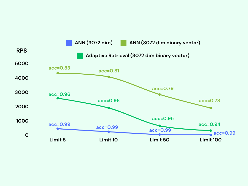
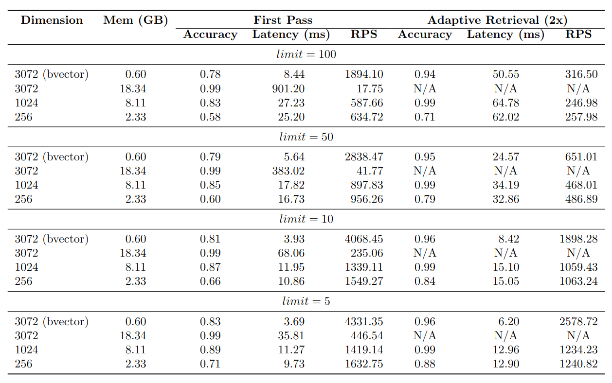
The results of the experiment are shown here:
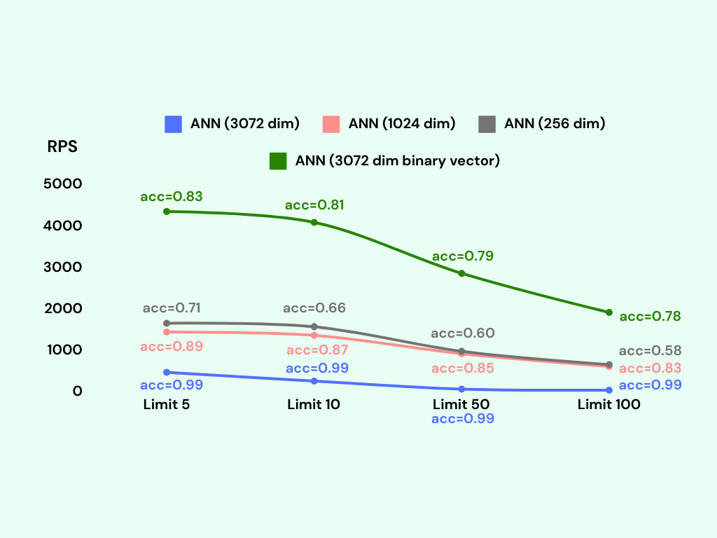
As anticipated, the 3072-dimensional embeddings exhibit the highest accuracy, while the 1024-dimensional embeddings demonstrate a slightly lower accuracy at around 85%. The 256-dimensional embeddings yield the lowest accuracy, approximately 65%. On the other hand, the binary vector index achieves an accuracy of about 80%.
Regarding the Requests Per Second (RPS) metric, the binary vector index showcases the most efficient performance, followed by the 256-dimensional embeddings, the 1024-dimensional embeddings, and finally, the 3072-dimensional embeddings.
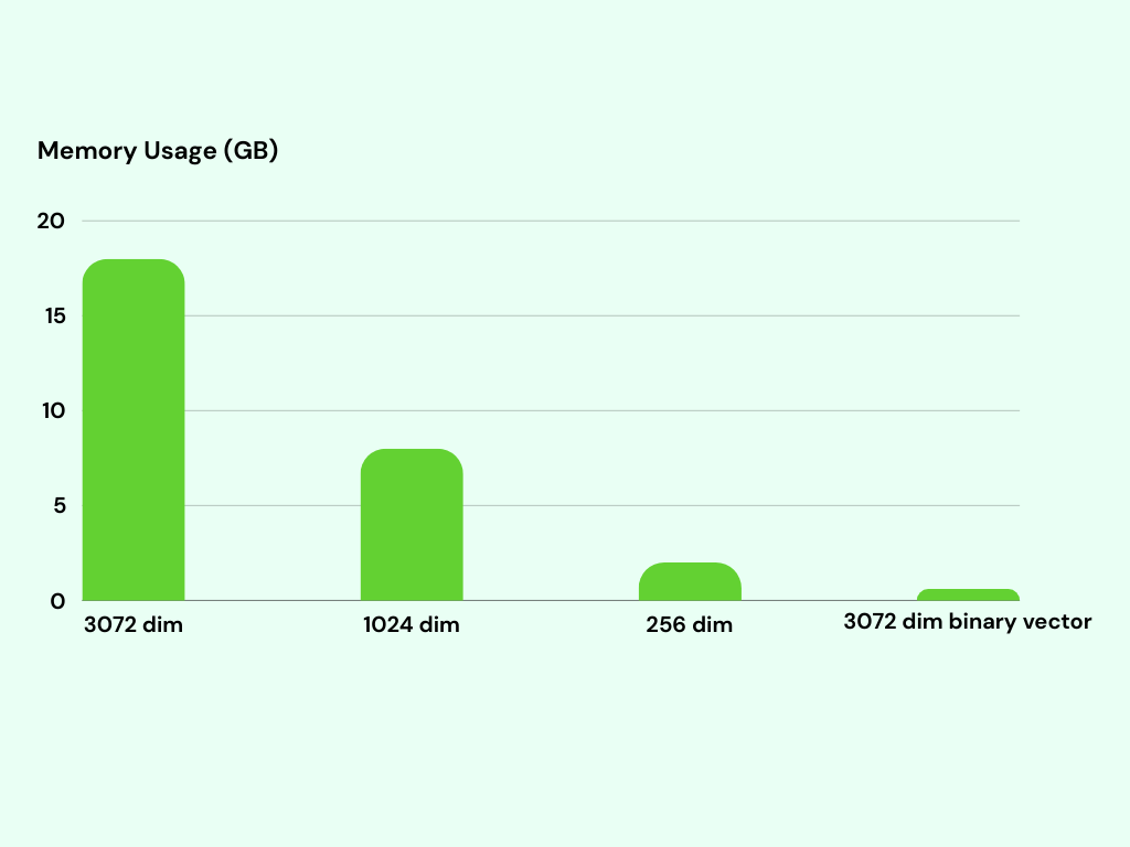
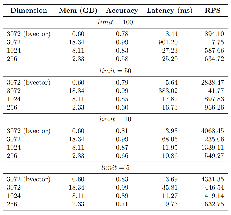
The memory usage of the indexes is an important aspect to take into account. Indexing 1 million 3072-dimensional binary vectors requires only around 600MB of memory. In contrast, the 3072-dimensional vector index consumes approximately 18GB of memory. This represents a significant difference in memory usage, as the 3072-dimensional vector index utilizes approximately 30x more memory than the binary vector index.
Improve the accuracy via adaptive retrieval
Lower dimension and binary vector indexes trade off accuracy for advantages such as higher RPS and lower memory usage compared to full dimension indexes. Adaptive retrieval techniques can be used to combine the strengths of both approaches, achieving an optimized solution that balances accuracy, memory usage, and query speed.
The logic behind adaptive retrieval is really simple. Let’s take get top 100 candidates as an example. We can perform the following steps:
- Query the lower dimensional or binary vector index first to retrieve 200 candidates from the 1 million embeddings. This is a fast operation.
- Rerank the candidates using a KNN query to retrieve the top 100 candidates. K-NN is well-suited for situations where smaller sets and precise similarity search are necessary, making it an excellent choice for reranking in this context.

The reranking step is a bit slower than the initial query, but it is still much faster than querying the full dimension index. It could be done in the pgvecto.rs:
The match_documents_adaptive function accepts a query embedding and a match count as input parameters. It first retrieves match_count * 2 candidates from the 1 million embeddings using the 256-dimensional index. Then, it reranks the candidates using a KNN query to retrieve the top match_count candidates.
The function for binary vector and 1024-dimensional embeddings can be implemented in a similar manner.
We conduct the benchmark again with the adaptive retrieval technique. We tag the adaptive retrieval technique as Adaptive Retrieval in the following figure.
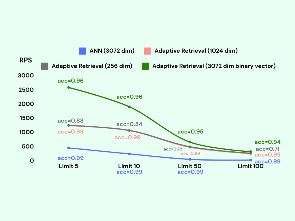
Adding a reranking step significantly improves the accuracy of the lower dimensional and binary vector indexes.
The binary vector index with adaptive retrieval achieves an accuracy of around 95%, with only a slight decrease in RPS compared to the binary vector index without adaptive retrieval. Remarkably, the memory usage of the binary vector index with adaptive retrieval is only around 600MB, which is the same as the binary vector index without adaptive retrieval.
Conclusion
Shortening embeddings can reduce the memory usage to store the embeddings, and speed up indexing and search. However, the accuracy of the shortened embeddings is not as good as the full embeddings. That’s why we need to use adaptive retrieval techniques to improve the accuracy of the lower dimensional indexes.
It seems that binary vector indexes with adaptive retrieval are the best choice for the text-embedding-3-large model. You could also consider 1024-dimensional indexes with adaptive retrieval if you need a higher accuracy (e.g. 99%).
PS: All the code and data used in this experiment are available in the pgvecto.rs-matryoshka-embeddings-benchmark.
3.3 - Image Search
Image intelligent search, also known as content-based image retrieval, goes beyond traditional keyword-based search and enables users to search for images based on their visual content. For example, you could search images that contain a red mushroom (image from immich):

The feature looks like a magic because it allows you to search for images that you don’t have keywords for. The search engine understands the content of the images and videos and can find the ones that are similar to the query.
How it works
Image intelligent search leverages advanced computer vision techniques and machine learning algorithms to understand the visual characteristics and features within images, allowing users to perform freeform searches without relying on specific keywords or metadata.
The first step is to extract meaningful features from images and generate a vector representation of each image. This is typically done using deep learning models such as CLIP. The vector representation is called an embedding. It is a list of numbers that represents the image.
Then you could use vector stores like pgvecto.rs to store the embeddings and perform efficient vector search.
Example
We will leverage CLIP, a neural network that connects text and images, to generate embeddings for our images. These embeddings capture the visual concepts present in the images. Subsequently, we will utilize pgvecto.rs, a scalable vector search tool built on Postgres, to store these embeddings and conduct efficient vector searches. By combining the power of CLIP and pgvecto.rs, we can retrieve similar images based on their visual content.
Generate embeddings
You could use CLIP to generate embeddings for images:
Store embeddings
Let’s say you have a table named images with three columns: id, author and embedding. The column embedding is of type vector(512). You could insert an image into the table like this:
Search for similar images
You could search for similar images like this:
Advanced search
Assuming you want to search for the 64 nearest rows and the results don’t contain the images from the author Allen.
You may want the following SQL to work:
In base mode, you may only get 32 rows since the HNSW algorithm bypasses filter conditions during the search and relies on PostgreSQL to apply filters post-search.
You could use the vbase search mode to achieve this. In vbase mode, searching results become an iterator that continuously returns results. The database can continuously retrieve results from it until the user’s query conditions are met. It’s quite different from other vector search library, such as faiss. The latter can only return a fixed-size result set, and this size needs to be determined before the search. For queries with filtering conditions, it is not possible to determine the size of the result set in advance. As a result, either insufficient results can be obtained or excessive searching will affect latency. The original idea comes from VBASE: Unifying Online Vector Similarity Search and Relational Queries via Relaxed Monotonicity.
You can enable vbase by a SQL statement SET vectors.search_mode = vbase;. Then you can get the correct behavior. This mode is used in immich’s image search feature. vbase is the default search mode in 0.2.
Real-world applications
Image intelligent search is used in immich to enable users to search for images based on their visual content. The code snippets provided here are inspired by the implementation of the image search feature in immich.
The query retrieves data from the asset_entity, smart_search, and exif_info tables based on specified conditions and ordering. Let’s break down the query:
This part of the query specifies the columns to be selected from the tables asset_entity, smart_search, and exif_info. The aliases a, s, and e are used to refer to each table respectively.
Here, the asset_entity table is aliased as a, the smart_search table as s, and the exif_info table as e. The INNER JOIN is used to combine asset_entity and smart_search based on the condition s.assetId = a.id. The LEFT JOIN is used to include matching records from the exif_info table based on the condition e.assetId = a.id.
The table asset_entity has the following schema.
In this part, the query applies filters to the asset_entity table. It selects rows where the ownerId column is among the specified userIds, isArchived is false, isVisible is true, and fileCreatedAt is earlier than the current time (NOW()).
The query orders the results based on the embedding column of the smart_search table, comparing it to the provided :embedding value. The <=> operator is used for the comparison.
Finally, limit the number of rows returned by the query to the value specified by the :numResults parameter.
This is an real-world use case to show how image intelligent search is implemented in a production system.
3.4 - Multi Tenancy
Multi-tenancy is essential for SaaS applications, allowing a single instance to serve multiple users or groups while ensuring data privacy and security. This blog outlines the design and implementation a simple multi-tenant vector search system with pgvecto.rs.
Designing the Database Schema
The success of user-based isolation in multi-tenant systems hinges on a well-structured database schema:
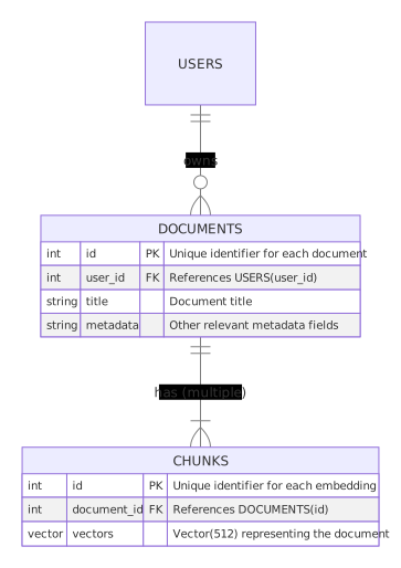
Users and Documents
Each user is identified by a unique user_id, which directly links them to their documents for private access. The documents table contains each user’s documents, each with a distinct id, title, and content. Additional metadata can be included in the documents table to improve search functionality. The user_id is linked to the documents instead of chunk embeddings to replicate real-world scenarios more accurately.
Chunks
Embeddings store vectorized representations of chunks of documents, and use document_id to reference its document.
Entity-Relation Diagram
Implementing Multi-Tenancy
Create Index
Create vector index on chunks.embedding to accelerate query process. Here we use dot product as the similarity measure.
Run the query with user_id
In this query:
- The
SELECTstatement now includes chunks.id AS chunk_id, documents.id AS document_id, and documents.title to return the chunk ID, the document ID, and the document title, respectively. - The
INNER JOINensures that only chunks associated with documents owned by the specified user (‘alice’) are considered. - The
ORDER BYclause calculates the distance between the chunk’s embedding and the provided vector [3,2,1], sorting the results by similarity. The closest or most similar embeddings are returned first. - Replace
[3,2,1]with the query embedding and ‘specific_user_id’ with the actual ID of the user for whom you are performing the search.
Performance Tip
The vector search will scan through additional points and evaluate the conditions individually. Consequently, if there is a large number of user IDs or the filter criteria are challenging to meet, the query speed may be impacted. To enhance performance, you may want to explore utilizing PostgreSQL’s partition table function.
3.5 - Sparse Vector Search
In the past, hybrid search combined two search methods: traditional keyword-based search and vector-based similarity search. However, sparse vector can act as a substitute for keyword search, unlocking the full potential of the data pipeline with pure vector search.
For more information about keyword-based hybrid search, please refer to Hybrid Search
This post explores how to use how BGE-M3 and pgvecto.rs to exploit the potential of hybrid search using both sparse and dense vectors.
Let’s dive in.
An Overview of Sparse and Dense Vector Embedding
Sparse vectors are high-dimensional vectors that contain few non-zero values. They are suitable for traditional information retrieval use cases. For example, a vector with 32,000 dimensions but only 2 non-zero elements is a typical sparse vector.
Dense vectors are embeddings from neural networks. They are generated by text embedding models and have most or all elements non-zero. They have fewer dimensions, such as 256 or 1536, much less than sparse vectors.
Dense vectors and sparse vectors are both used to represent features of text chunks, but they have significant differences. A single dimension in a dense vector embedding does not mean anything, as it is too abstract to determine its meaning. However, when we take all the dimensions together, they provide the semantic meaning of the input text.
Sparse vectors have dimensions equal to the vocabulary size, with each element representing the weight of a word in the text.
Generally, words with higher weights indicate greater importance in the text. Sparse vectors simplify the analysis and visualization of the relationship between text and vocabulary. To visualize dense vectors, additional dimension reduction algorithms are necessary, such as:
- Principal component analysis (PCA)
- T-distributed stochastic neighbor embedding (T-SNE)
- Uniform Manifold Approximation and Projection (UMAP)
| Dense Vector | Sparse Vector | |
|---|---|---|
| Dimension | Hundreds to thousands | Tens of thousands |
| Element Meaning | Nothing | Word Weight |
| Interpretability | Hard | Easy |
| Usage | Vector Distance | Vector Distance / Visualize |
| Semantic sensitivity | High | Low |
Sparse vectors are generally less effective at capturing the relationships between words, particularly for synonyms and related terms, compared to dense vectors.
For instance, both rocket and SPACE X are related to space exploration, but Dense vectors are more likely to reveal similarities and assign a closer vector distance to corresponding texts.
How to create a vector embedding?
A vector embedding is the internal representation of input data in deep learning models, also known as embedding models. Most embedding models, such as text-embedding-3-small, only output dense embeddings.
SPLADE and BGE-M3 can generate sparse embeddings, sometimes called lexical weights. In this section, we will introduce the BGE-M3 model for generating dense and sparse vectors.
BGE-M3 is a multi-functionality model, which can simultaneously perform the three common retrieval functionalities of the embedding model: dense retrieval, multi-vector retrieval, and sparse retrieval. We will learn how to generate dense and sparse embeddings from it.
For all sentences and words, a text-word matrix was created:
| TEXT | What | is | BM | 25 | ? | Definition | of | … |
|---|---|---|---|---|---|---|---|---|
| What is BM25? | 0.08 | 0.08 | 0.13 | 0.25 | 0.04 | 0 | 0 | … |
| Definition of BM25 | 0 | 0 | 0.25 | 0.33 | 0 | 0.14 | 0.06 | … |
The matrix is highly sparse, especially when all vocabularies are included. Most words only appear in a few sentences, resulting in non-zero weights.
By feeding text into sparse embedding models like BGE-M3, we can easily obtain sparse embeddings from it.
Now we have both the sparse and dense embeddings. It’s time to insert them into the vector database.
Storing vectors in pgvecto.rs
First, a deployed pgvecto.rs instance is required for vector storage and retrieval. This can be achieved by the official pgvecto-rs Docker image:
Now the only necessary dependency is installed. Let’s create a table to store the vectors.
pgvecto.rs supports dense or sparse vectors with different data types:
vectorfor dense vectorsvectorfor sparse vector
The BGE-M3 model has a dense embedding dimension of 1024. The sparse embedding dimension is 250002, which matches the size of tokenizer vocabulary.
In this example, we create a table named documents with four columns: an ID column(id), a text column(text) and two vector columns(sparse for sparse vector and dense for dense vector).
With the table created, we can now insert embeddings into the table and create indexes for vector columns.
For dense vectors, vector_l2_ops calculates the Squared Euclidean distance, which is the most commonly used distance metric.
For sparse vectors, vector_dot_ops calculates the dot product, which is a more efficient method.
For more information about index types in pgvecto.rs, please check out our documentation.
Retrieving and Mixing Results
With the vectors stored in the database, we can efficiently query them using the pgvecto.rs extension. To find the nearest vectors to a given input text, we need to encode the text with the same model.
This process is identical to the one described in the previous chapter:
The pgvecto.rs extension provides a simple SELECT statement to get sparse and dense vectors like this:
To rerank the merged result, you can use popular fusion methods such as Reciprocal Ranked Fusion (RRF). However, to make better use of BGE-M3, let’s introduce the Reranker model of BGE-M3. Unlike the embedding model, Reranker uses text input and directly outputs their similarity or score.
We can initialize a Reranker model and feed it with mixed candidate texts. With this method, reranking can be as simple as sorting by the Reranker model’s estimated score.
Congratulations! We have now completed our first step into the world of sparse vector search.
3.6 - Generative Question-Answering
Vector search can also be used to provide context to generative models such as OpenAI’s GPT series, improving the quality of the outputs.
This post will explore the use of pgvecto.rs in building and retrieving from a vector knowledge base to bolster the performance of generative models in question-answering tasks. A knowledge base serves as “long-term memory” for generative models, providing them persistent, curated, and accurate information as context to draw from when generating an answer to a question. This results in answers that are more accurate, reduces the possibility of the model producing “hallucinations” (statements with no basis in reality), and increases user trust in the outputs. This technique is known as Retrieval-Augmented Generation, or RAG: see this post or the related paper for more information.
Overview of the Question-Answering task
The generative model question-answering (QA) task is a method of Information Retrieval. The model is presented with a question, and generates an answer based on some context: typically, documents or other information sources the model can look at to retrieve the information necessary to answer the question.
This use case will involve giving the OpenAI gpt-3.5-turbo-instruct model context to answer questions about movies from the vishnupriyavr/wiki-movie-plots-with-summaries-faiss-embeddings Huggingface dataset.
The overall workflow will look something like this:
Question-Answering without Context
First, let’s try having the model answer some questions without providing it context.
We begin with defining a function to streamline getting a response for a given prompt:
The api_key requires an OpenAI account. Once logged in, sign up for an API key from the top-right drop-down menu, and paste it in place of YOUR_API_KEY_HERE.
Let’s start with asking about a relatively popular movie:
The release year of Skyfall is 2012. The overall plot follows James Bond as he investigates an attack on MI6 and uncovers a sinister plot by a former agent seeking revenge on M and the entire agency. Bond must confront his past and protect MI6 from destruction.
Accurate, if somewhat vague in the plot summary. However, what about a movie that’s much less known?
The release year of Cat Napping is unknown. The overall plot of Cat Napping is about a group of cats who go on a mission to rescue their friend who has been kidnapped by a group of evil dogs. Along the way, they encounter various challenges and obstacles, but with their cleverness and teamwork, they are able to save their friend and defeat the dogs.
Cat Napping is actually a Tom and Jerry movie from 1951, where the two fight over a hammock.
We have found the limits of what the model “knows”: it is unable to produce the release year, and invents a potential plot based on the title. We will remedy this by creating a knowledge base for the model to draw on.
There are two options for allowing the model to better answer our question:
- Fine-tune the model on text data in the domain of interest (movies in this case).
- Employ retrieval augmented generation, which adds an information retrieval component to the process. This will allow us to retrieve and feed relevant information to the model as a secondary source of information.
We will be taking the second option in this post.
Building the Knowledge Base
Let’s build a knowledge base of movies to retrieve relevant information from, using the vishnupriyavr/wiki-movie-plots-with-summaries-faiss-embeddings Huggingface dataset. This dataset contains titles, release years, casts, Wikipedia pages, plot summaries/lengths, and vector embeddings of this information for 33,155 movies. Each movie also has text data, which encompasses title, release year, cast, and plot summary in one. We will be using the text and embeddings data for this application.
Load the Data
Start by loading the data:
Generate Embeddings
This particular dataset comes with embeddings, so you can skip this step and use the embeddings directly.
If you want to generate embeddings from the text data, you can use the OpenAI, Cohere or other embeddings APIs. We provide an example using the Cohere API, you can get Cohere API key from here.
The embeddings in this user case are dense vectors. For creating sparse vectors, you can see this page.
Insert Data into the Database
A deployed pgvecto.rs instance is required for vector storage and retrieval. We can use the official pgvecto-rs Docker image:
Install the required psycopg library to interact with Postgres, and ensure the extension is running:
Now, we create a table movies with a few columns: an ID column(id), a text column(texts), and a vector column(embeddings).
We use type vector(n), as we are working with dense vector embeddings, where n is the dimension of each embedding (768 in this case).
With the table created, we can now insert the embeddings from the dataset and create indexes for vector columns:
This may take a while, depending on how much data is to be inserted.
Create Index
Recall that for dense vectors, vector_l2_ops calculates the Squared Euclidean distance, which is the most commonly used distance metric.
$$
D_{L2} = \Sigma (x_i - y_i) ^ 2
$$
Question-Answering with Context
To make use of our knowledge base, queries must first be encoded to determine what texts to retrieve:
Now, we define a function to streamline adding the retrieved context to the initial prompt:
Recall the options for distance operators:
<->for squared Euclidean distance<#>for negative dot product<=>for cosine distance
For definitions, please see the overview.
Now, let’s try the prompt again, with added context:
The release year of Cat Napping is 1951 and the overall plot involves Tom and Jerry fighting over a hammock, with Jerry ultimately getting revenge on Tom.
Now the model has given us a more accurate answer! We can even ask further questions:
Tom tries to send Jerry sliding into a nearby pond by unhooking the hammock he is sleeping in. He also tries to whack the hammock to send Jerry flying into the air, but Jerry lands in a bird’s nest. Tom then picks Jerry up on a spatula and places him onto a walking army of ants, causing Jerry to wake up as he bumps his head on a sprinkler. Tom also tries to chase Jerry with a lawn mower and a baseball bat.
As we saw earlier in this post, LLMs do work very well by themselves, but can struggle with niche or specific questions, creating “hallucinations” that may not be noticed. The use of the knowledge base improves factuality and subsequently user trust in the generated outputs.
Further Applications
This method is not only for asking about movies, of course. Other applications could include extracting summaries of scientific papers (try this dataset!), or answering questions about company policies provided a database of company literature.
4 - Integration
4.1 - LangChain
This document describes the LangChain integration.
LangChain is a framework for developing applications powered by language models. It is a set of tools that allows you to fine-tune, deploy, and use language models in production.
pgvecto.rs provides a LangChain integration that allows you to retrieve the most similar vectors in LangChain.
Install dependencies
Some dependencies are required to use the LangChain integration:
You could start the postgres instance with pgvecto.rs extension in a docker container:
Then you can connect to the database using the psql command line tool. The default username is postgres, and the default password is mysecretpassword.
Run the following SQL to ensure the extension is enabled.
Create the database and load documents
We will show how to use pgvecto.rs in LangChain to retrieve the most similar vectors.
First, you need to create the text loader and the text splitter to split the text into chunks. We use the markdown file getting-started/overview.md as an example.
Then, we will create the PGVecto_rs instance and load the documents into the database.
Query index
Finally, we can retrieve the most similar chunks in LangChain.
The output is:
Initialize from an existing database
Above, we created a vector store from scratch. However, often times we want to work with an existing vector store. In order to do that, we can initialize it directly.
Then, we can add vectors to the store and query:
The output is:
4.2 - LlamaIndex
LlamaIndex is a simple, flexible data framework for connecting custom data sources to large language models (LLMs).
pgvecto.rs provides a LlamaIndex integration that allows you to retrieve the most similar vectors.
Install dependencies
Some dependencies are required to use the LlamaIndex integration:
You could start the postgres instance with pgvecto.rs extension in a docker container:
Then you can connect to the database using the psql command line tool. The default username is postgres, and the default password is mysecretpassword.
Run the following SQL to ensure the extension is enabled.
Create the database and load documents
First, create the text loader and the text splitter to split the text into chunks. We use the markdown file getting-started/overview.md as an example.
Then setup the OpenAI API key and load the documents into the database.
Query index
Finally, we can retrieve the most similar chunks.
4.3 - Citus
citus is a PostgreSQL extension that turns Postgres into a distributed database. pgvecto.rs works well with citus Here are the steps to enable vector search in a distributed PostgreSQL instance.
citus can works on Single-Node and Multi-Node, both of which are compatible with pgvecto.rs natively.
Single-Node Citus
First, prepare the dockerfile with pgvecto.rs and citus installed and attach them to PostgreSQL.
citus must be placed first in shared_preload_libraries due to its restrictions.
Then we will build a Docker image called citus-vector:16 locally.
Don’t use POSTGRES_HOST_AUTH_METHOD: "trust" in production, see citus notes about Increasing Worker Security for detailed authentication configure.
To enable the essential extensions, connect our container with psql and execute SQL command.
Once the extensions are created, you can create a simple table, then transform it into a distributed table.
The index build and vector search is as same as before. Tables and indexes are distributed to all shards/workers automatically.
Multi-Node Citus
You can use the same Dockerfile and image for Multi-Node citus as for Single-Node Citus.
In this example, we will start a cluster of 1 coordinator node and 2 worker nodes with docker compose.
Don’t use POSTGRES_HOST_AUTH_METHOD: "trust" in production, see citus notes about Increasing Worker Security for detailed authentication configure.
Now start all containers with docker-compose. Each container is a citus node, with 1 coordinator(main) and 2 workers.
As before, you’ll want to enable the extensions, but make sure you run the command on all nodes.
To inform the coordinator about its workers, connect to the coordinator node with psql and register the two workers.
Finally, you can perform vector queries in the same way as in Single-Node Citus.
Monitor
If you’re using a citus distributed table, the pg_vector_index_stat view on the coordinator will be empty. Since all the indexes are created at the workers actually, we can only inspect the vector status by distributing this view to the workers.
5 - Administration
5.1 - Configuration
Logging
By default, you cannot capture all pgvecto.rs logs. pgvecto.rs starts a background worker process for indexing, and it prints logs to standard error. To capture them, you need to set logging_collector to on. You can get more information from PostgreSQL document about logging collector.
You can set logging_collector to on with the following command:
Index configuration
since v0.3.0For each index, there are a number of configuration items that are variable. Unlike options, they support real-time modification after the index has been created. These items can be configured by function alter_vector_index.
Here are all the available configurations.
Threads for backend optimizing
By default, each vector index is optimized by only one thread at the backend. However, if you have multiple idle CPUs and want to take advantage of them, you can increase the number of threads.
Set the key argument to optimizing.threads and the value argument to the desired number of threads.
5.2 - Upgrading
General Steps
If you update the extension to a new version, let’s say it’s a.b.c. This command helps you to update the schema of extension:
If you’re upgrading from 0.1.x, please read Upgrading from 0.1.x.
If you’re upgrading to 0.4.0, please read Upgrading to 0.4.0.
Execute the following SQL. It helps you do some maintenance work.
You need to restart PostgreSQL to take effects.
You could check the status of all vector indexes in this command:
Let’s assume the output is:
Then you could reindex all vector indexes.
Upgrade to 0.4.0
You may get this error if some indexes were created before upgrading pgvecto.rs to 0.4.0:
You can simply drop these indexes, and then upgrade the extension:
Upgrade from 0.1.x
You need to follow these steps to make ALTER EXTENSION vectors UPDATE work.
Let’s assume your pgvecto.rs version is 0.1.x (replace x with a number).
pgvecto.rs is installed in schema vectors from 0.2.0, you may need to set search_path for the database.
5.3 - Logical replication
Logical replication is a feature in PostgreSQL that enables the replication of individual database objects or a subset of data from one PostgreSQL database to another.
With logical replication, you can selectively replicate specific tables, databases, or even specific rows based on predefined replication rules. This provides more flexibility compared to physical replication, where the entire database cluster is replicated. It allows you to design custom replication topologies and replicate only the data that is necessary for your use case.
We will show you how to use logical replication to replicate data from one PostgreSQL database to another.
Deploy source and target PostgreSQL clusters
Create extension vectors in source database and target database.
Configure logical replication
Now, we can set logical replication between source database and target database.
Prepare test data
We need to create a table named test with a column named embedding of type vector(10) in source database and target database. Then we create an index on the embedding column of the test table in source database and target database. Finally, we insert data into the source database.
Create the table
Create the index
We create an index on the embedding column of the test table in source database and target database. The index type is flat, it is a brute force algorithm. We choose vector_l2_ops squared Euclidean distance to measure the distance between vectors. Another index type and distance function can be found in here.
Insert data
We only need to insert data into the source database. The data will be synchronized to the target database.
In source database, now you can search for the nearest neighbor of a vector in the embedding column of the test table.
If you query the target database, you will get the noting:
Set up logical replication
To simplify the process of setting up logical replication between two PostgreSQL databases, we will use pg-easy-replicate.
We use pg-easy-replicate to set up logical replication between source database and target database.
Bootstrap
Every sync will need to be bootstrapped before you can set up the sync between two databases. Bootstrap creates a new super user to perform the orchestration required during the rest of the process. It also creates some internal metadata tables for record keeping.
Start sync
Once the bootstrap is complete, you can start the sync. Starting the sync sets up the publication, subscription and performs other minor housekeeping things.
Test logical replication
Query
Now we can query the target database to get the nearest neighbor of a vector in the embedding column of the test table. The result is the same as the source database.
Update index
If you insert data into the source database, the data will be synchronized to the target database. Insert data into the source database:
Query in the source database:
Query in the target database, it will return the same result:
5.4 - Foreign data wrapper (FDW)
Foreign data wrapper(FDW) is an extension in PostgreSQL that allows you to access and query data stored in remote databases as if they were local tables. FDW provides a way to integrate and interact with different data sources.
With the FDW extension, you can define foreign tables in your local PostgreSQL database that mirror the structure of tables in remote databases. These foreign tables act as proxies or wrappers for the remote data, enabling you to perform SELECT, INSERT, UPDATE, and DELETE operations on them, just like regular tables in PostgreSQL.
In this tutorial, we will use the postgres_fdw module, which includes the foreign-data wrapper. This wrapper can be used to access data stored in external PostgreSQL servers. This article will explain how to use postgres_fdw to access index data in a foreign PostgreSQL cluster that already has the pgvecto.rs extension installed.
Deploy local and foreign PostgreSQL clusters
In this tutorial, we will use docker compose to deploy two PostgreSQL clusters.
Foreign database operations
First, we need create a table test and build an index on it in the foreign db. The test table has two columns: id and embedding. The embedding column is a vector column, and its type is vector(10). The id column is the primary key of the test table.
Create a table
Create a user
Create a user named fdw_user in foreign db, and grant SELECT, INSERT, UPDATE, DELETE privileges on table test to fdw_user.
Create the index
We create an index on the embedding column of the test table. The index type is flat, it is a brute force algorithm. We choose vector_l2_ops squared Euclidean distance to measure the distance between vectors. Another index type and distance function can be found in here.
Local database operations
In local database, we need to create a table local and a foreign server foreign_server. The local table has two columns: id and name. The id column is the primary key of the local table. The foreign_server is a foreign server, which is used to access the foreign db.
Create local table
create local user
Using superuser, execute the following statement in the local PostgreSQL database to create a regular user named local_user.
Create the foreign server
To create an external server using the CREATE SERVER statement, you need to specify the host, port, and database name of the remote database.
Create the user mapping
Use the CREATE USER MAPPING statement to create a mapping between remote users and local users, requiring the username and password of the remote user.
Creat the foreign table
Use the CREATE FOREIGN TABLE statement to create a remote table. It is important to note that the types of each column should match those of the actual remote table, and it’s best to keep the column names consistent. Otherwise, you will need to use the column_name parameter to specify the column name in the remote table for each individual column.
Authorization
Authorize the local_user:
- Grant
local_userthe permission to use postgres_fdw. - Grant
local_userthe permission to use foreign serverforeign_server. - Grant
local_userthe permission to access all tables in schemapublic.
Query
Now we can use join query to access the foreign table in local db.
5.5 - Kubernetes
If you want to use pgvecto.rs in PostgreSQL which is running in Kubernetes, we provide a tutorial to help you. In this tutorial, we will use CloudNative-PG to deploy PostgreSQL cluster in Kubernetes.
Requirements
| Name | Version |
|---|---|
| helm | >= 2.4.1 |
| kubectl | >= 1.14 |
| Kubernetes | >= 1.24.0 |
Install CloudNative-PG
We use CloudNative-PG (cnpg) to deploy PostgreSQL cluster in Kubernetes. You can install it by helm.
Build PostgreSQL image with pgvecto.rs
We use the official CloudNative-PG docker image as the base image, and install pgvecto.rs in it. And you can also find pgvecto.rs version from releases.
Notice: PostgreSQL docker image tag must start with CNPG_TAG for cloudnative-pg to recognize the postgres version.
Create PostgreSQL cluster
We provide a sample yaml file to create a PostgreSQL cluster in Kubernetes. You can modify it according to your needs. You need pay attention to the following points:
- Set
shared_preload_librariesto loadpgvecto.rsshared library. You can also setpostInitApplicationSQLALTER SYSTEM SET shared_preload_libraries = "vectors.so";to loadpgvecto.rsshared library. - Execute
CREATE EXTENSION IF NOT EXISTS "vectors";to createvectorsextension.
You can install cnpg kubectl plugin to manage your PostgreSQL cluster. Now we can check the status of the cluster.
Notice: This article just provides a minimal configuration, not include logical replication, streaming logical replication, backup and restore, etc. We will provide those in another article. You can also refer to CloudNative-PG for more
Clusterconfiguration.
Connect to PostgreSQL cluster
You can use kubectl port-forward to connect to PostgreSQL cluster.
The vectors extension is installed successfully. You can try quick-start without installation.
5.6 - Migration
outline: [2,3]
PGVecto.rs Migration Overview
From pgvector
Prerequisites
When migrating from pgvector to PGVecto.rs, it is possible that you may have a table with a column of vector type. An example of this would be:
In addition, some rows will be inserted into the table, as follows:
In most cases, there will also be one or more vector indexes:
This is a typical scenario when pgvector is used. If the following requirements are met, the migration can be initiated.
- Please note that your
pgvectorextension is not installed in thevectorsschema. This means that you can installpgvectorandPGVecto.rsat the same time.
Steps to Migration
1. Install PGVecto.rs
Please follow the instructions provided to install PGVecto.rs and ensure that the extension is loaded by PostgreSQL.
The two extensions, pgvector and PGVecto.rs, are now installed at the PostgreSQL.
To validate the install, please run \dx in psql. You will see that there is an extension called vector for pgvector and another called vectors for PGVecto.rs.
Please note that there are some symbols with the same name in both extensions. This may cause confusion when doing the migration. To differentiate between the two, please verify that the search_path does not include the PGVecto.rs schema vectors.
2. Check existing indexes
For indexes created at vector columns, please retrieve the definition and record it in a convenient location. This information is necessary for the recovery of the indexes at a later stage.
3. Migrate vector columns
To migrate from a pgvector vector column, the first step is to create a PGVecto.rs vector column of the corresponding type. The subsequent step is to replicate the vector data from the original column to the new one.
Here provides the conversion path for each vector type of pgvector:
vector(pgvector) -> real[] -> vector(PGVecto.rs)halfvec -> vector(pgvector) -> real[] -> vector(PGVecto.rs) -> vecf16bit -> text[] -> real[] -> vector(PGVecto.rs) -> bvector
This vector type is not supported for migration yet:
sparsevec
Method 1: Conversion after validation
With this method, you can check the correctness of the vector data during the migration process, and you do not need to worry about the indexes that have been created on the vector columns, as they will be automatically deleted. However, it requires additional memory to store the vectors before and after the migration.
This step will cause some downtime, due to:
- a short
ACCESS EXCLUSIVElock byALTER TABLE ADD COLUMN - a much longer
ROW EXCLUSIVElock byUPDATE - a short
ACCESS EXCLUSIVElock byALTER TABLE DROP COLUMN
Once the data has been copied, you can check the data by SELECT and replace the existing column with the new one.
Method 2: Conversion without additional memory
With this method, the migration will be completed in one command and no additional memory is required. However, you need to delete the index on the vector column in advance.
This step will cause some downtime, due to:
- a long
ACCESS EXCLUSIVElock byALTER TABLE ALTER COLUMN
4. Recreate index
To recreate index on vector columns for PGVecto.rs , please enable the compatibility mode and create it like before.
For other vector types, such as halfvec, sparsevec, and bit, please refer to the indexing. Currently, pgvector_compatibility mode is not supported for these types.
5. Clean the environment
You may now safely remove the pgvector extension if it is no longer required.
In the event that the pgvector extension is removed, it is advisable to reset the search_path in order to ensure that symbols in PGVecto.rs are accessible globally.
Verify the result
Once the migration task is executed, you can verify the new columns by SELECT SQL.
6 - FAQs
6.1 - General FAQ
We strongly suggest you explore our new VectorChord implementation, offering enhanced stability and performance. Users are advised to transition to VectorChord. Refer to the migration guide for assistance.
The vector type or operator class is not found
In most cases, this is due to a missing schema search path or a lack of permissions.
Please go through this checklist:
- Run
\dxwithpsqlorSELECT * FROM pg_extension;and check if the extension exists.
If not, install it with CREATE EXTENSION vectors;
- Run
SHOW search_path;and check if it containsvectors.
If not, set it with SET search_path="$user", public, vectors;
- If
pgvecto.rsis installed by another superuser
Run \dn with psql or SELECT nspname FROM pg_catalog.pg_namespace; and check if the schema vectors exists.
If not, log in as the superuser and grant schema permissions to current_user:
GRANT ALL ON SCHEMA vectors to tensorchord;
6.2 - Comparison with pgvector
Original post: pgvector vs. pgvecto.rs in 2024: A Comprehensive Comparison for Vector Search in PostgreSQL
TL; DR: Please navigate directly to the final section that contains a table showcasing the main distinctions.
Search
Search is essential for a database. It plays a pivotal role in facilitating efficient data retrieval, enabling users to quickly find and access the information they need. We will demonstrate their performance and highlight the various features pgvecto.rs and pgvector offer.
Filtering
While both pgvector and pgvecto.rs provide support for vector similarity search in PostgreSQL, pgvecto.rs goes a step further by introducing VBASE method from OSDI 2023.
Real-world workloads often involve a combination of vector search and relational queries. While vector search is powerful for similarity matching and retrieval of similar vectors, relational queries allow you to perform complex joins, filters, and aggregations on structured data.
pgvecto.rs is designed to perform efficiently in scenarios that involve Single-Vector TopK + Filter + Join.
We utilize the laion-768-5m-ip-probability dataset for benchmarking purposes due to the absence of a comprehensive relational benchmark. The dataset is derived from LAION 2B images. It contains 5,000,000 vectors, 10,000 queries.
The dataset includes a probability column that stores random floating-point values generated from a uniform distribution between 0 and 1. The ratio of 0.01 means that each query covers 1% (or 0.01 times) of the dataset, allowing for focused analysis.
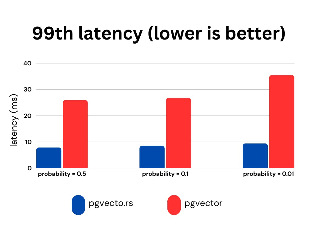
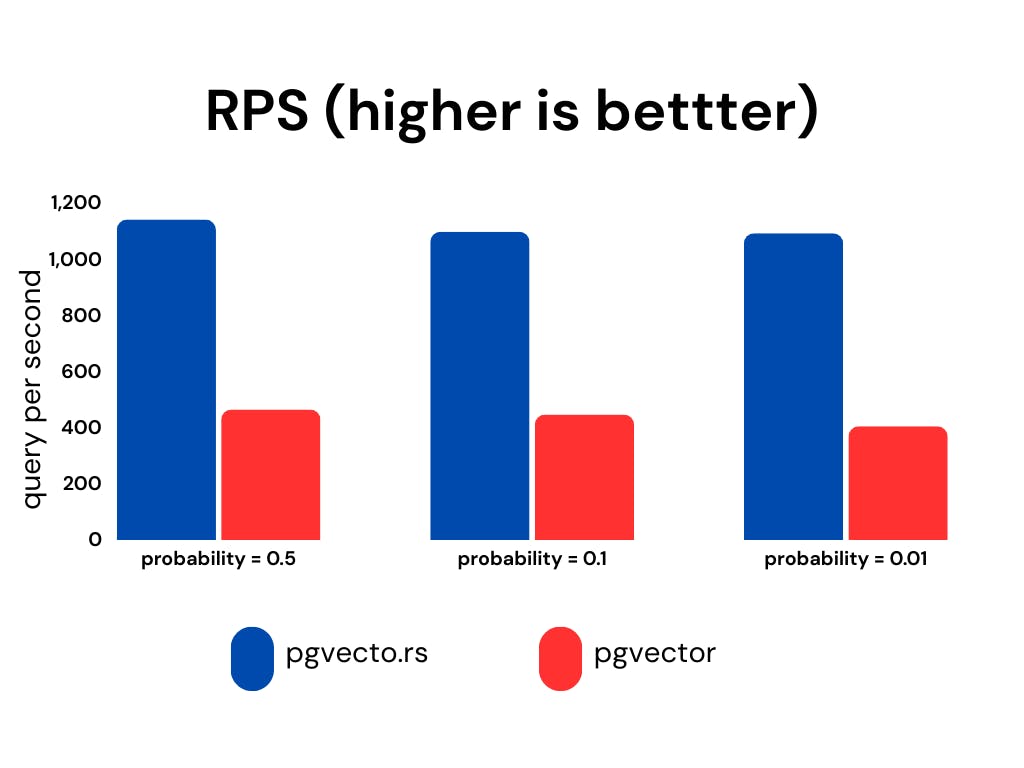
We present the recall, latency (in milliseconds), and RPS (requests per second) for various probability ranges while keeping the ef_search constant. The ef_search parameter represents the size of the list utilized during k-NN (k-Nearest Neighbors) searches, determining the trade-off between search accuracy and query processing time.
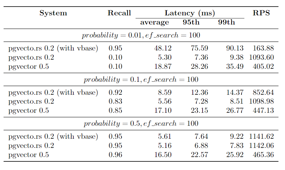
pgvecto.rs, when used with VBASE, consistently yields improved recall, particularly when working with low probability values.
Sparse Vector Search
Sparse vectors are high-dimensional vectors that contain few non-zero values. They are suitable for traditional information retrieval use cases. For example, a vector with 32,000 dimensions but only 2 non-zero elements is a typical sparse vector.
Dense vectors are embeddings from neural networks. They are generated by text embedding models and have most or all elements non-zero. They have fewer dimensions, such as 256 or 1536, much less than sparse vectors.
pgvecto.rs supports both dense vector search and sparse vector search. It provides the ability to use the svector data type to build sparse vector indexes and perform searches on them.
Vector dimensions
The pgvecto.rs extension provides support for up to 65535 dimensions, whereas the pgvector extension supports a maximum of 2000 dimensions. This difference in dimensionality support allows pgvecto.rs to handle vectors from OpenAI’s latest embedding model directly.
Single Instruction/Multiple Data (SIMD)
pgvecto.rs utilizes the SIMD (Single Instruction, Multiple Data) instructions available on the user’s machine, pgvector relies on the compiler to generate SIMD code at compile time and cannot choose a faster instruction set at runtime. It makes search in pgvecto.rs faster due to the faster calculation of vector distances.
Data Types
Binary Vector
The bvector type is a binary vector type in pgvecto.rs. It represents a binary vector, which is a vector where each component can take on two possible values, typically 0 and 1.
Binary vectors offer significant advantages in specific embedding models like the OpenAI embedding model by effectively reducing memory usage while preserving a satisfactory level of accuracy.
Here are some performance benchmarks for the bvector type. We use the dbpedia-entities-openai3-text-embedding-3-large-3072-1M dataset for the benchmark. The VM is n2-standard-8 (8 vCPUs, 32 GB memory) on Google Cloud.
We upsert 1M binary vectors into the table and then run a KNN query for each embedding. It only takes about 600MB memory to index 1M binary vectors, while the vector type takes about 18GB memory to index the same number of vectors. The bvector’s accuracy exceeds 95% if we adopt adaptive retrieval.
FP16/INT8
Besides binary vectors, pgvecto.rs also provides support for FP16 (16-bit floating point) and INT8 (8-bit integer) data types.
Indexing
pgvecto.rs takes a different approach compared to pgvector. It handles the storage and memory of indexes separately from PostgreSQL, instead of relying on the native storage engine of PostgreSQL like pgvector does.
It’s a design tradeoff. During the initial stages of our development, we conducted experiments with PostgreSQL’s page storage for the Hierarchical Navigable Small World (HNSW) index. similar to pgvector. However, we encountered various limitations that hindered its effectiveness and functionality:
- Parallelization Challenges: The process model of PostgreSQL, where each statement corresponds to a single process and the lack of thread-safe APIs, presents challenges for parallelization. In the case of building vector indexes, which involve computationally intensive tasks, parallelization can significantly enhance performance. However, our efforts to parallelize this process were impeded by frequent occurrences of ‘Too many shared buffer locked’ errors.
- Write-Ahead Logging (WAL) Amplification: The issue of Write-Ahead Logging (WAL) amplification arises when inserting a 2KB vector results in generating over 20KB of WAL. This problem is inherent in the HNSW algorithm used, as it involves modifying multiple edges for a single point insertion. PostgreSQL records each change individually in the WAL, leading to substantial amplification of the WAL size.
- Lock Contention: Lock contention arises due to the need to lock every edge list during reads and writes when traversing the HNSW graph. The hierarchical structure of HNSW, where higher levels contain fewer points, often results in lock contention becoming a common bottleneck during index usage. This contention occurs when multiple operations attempt to access or modify the same edge list simultaneously, leading to delays and reduced concurrency.
pgvecto.rs adopted a design akin to FreshDiskANN, resembling the Log-Structured Merge (LSM) tree concept. This architecture comprises three components: the writing segment, the growing segment, and the sealed segment. New vectors are initially written to the writing segment. A background process then asynchronously transforms them into the immutable growing segment. Subsequently, the growing segment undergoes a merge with the sealed segment, akin to the compaction process in an LSM tree. This design offers several benefits:
- Non-blocking Insertions: Index modification operations do not impede insertion processes.
- Batched Modifications: Grouping modifications to the HNSW graph improves throughput.
- Elimination of Read-Write Lock Contention: Since sealed segments are immutable, issues related to read-write lock contention are mitigated.
However, there are drawbacks to this approach. One notable limitation is the absence of out-of-the-box Write-Ahead Logging (WAL) support for the index. This means that features like Point-in-Time Recovery and Physical Replication, which rely on WAL, are not readily available for the index. Nevertheless, the PostgreSQL ecosystem is robust and allows for extensions to define their own custom WAL through a resource manager. While implementing this solution requires additional effort, it is feasible to overcome the limitation and enable WAL support for the index.
Summary
Here we will show the main distinctions between pgvecto.rs and pgvector.
| Feature | pgvecto.rs | pgvector |
|---|---|---|
| Filtering | Introduces VBASE method for vector search and relational query (e.g. Single-Vector TopK + Filter + Join). | When filters are applied, the results may be incomplete. For example, if you originally intended to limit the results to 10, you might end up with only 5 results with filters. |
| Vector Dimensions | Supports up to 65535 dimensions. | Supports up to 2000 dimensions. |
| SIMD | SIMD instructions are dynamically dispatched at runtime to maximize performance based on the capabilities of the specific machine. | Relies on compiler-generated SIMD code at compile time. |
| Data Types | Introduces additional data types: binary vectors, FP16 (16-bit floating point), and INT8 (8-bit integer). | - |
| Indexing | Handles the storage and memory of indexes separately from PostgreSQL | Relies on the native storage engine of PostgreSQL |
| WAL Support | Provides Write-Ahead Logging (WAL) support for data, index support is working in progress. | Provides Write-Ahead Logging (WAL) support for index and data. |
6.3 - Why not a specialty vector database?
Read our complete blog at Do we really need a specialized vector database? (2023) | vchord.pgsty.com.
Imagine this, your existing data is stored in a Postgres database, and you want to use a vector database to do some vector similarity search. You have to move your data from Postgres to the vector database, and you have to maintain two databases at the same time. This is not a good idea.
Why not just use Postgres to do the vector similarity search? This is the reason why we build pgvecto.rs. The user journey is like this:
From SingleStore DB Blog:
Vectors and vector search are a data type and query processing approach, not a foundation for a new way of processing data. Using a specialty vector database (SVDB) will lead to the usual problems we see (and solve) again and again with our customers who use multiple specialty systems: redundant data, excessive data movement, lack of agreement on data values among distributed components, extra labor expense for specialized skills, extra licensing costs, limited query language power, programmability and extensibility, limited tool integration, and poor data integrity and availability compared with a true DBMS.
6.4 - Benchmarks
pgvecto.rs has been focused on performance from the beginning. We have continuously monitored the performance of pgvecto.rs and compared it with other vector search libraries. The following benchmark results are from January 2024.
The test is done on Google Cloud n2-standard-8 (8 vCPUs, 32 GB RAM) with the laion-768-5m-ip dataset.
pgvecto.rs v.s. pgvector
With the HNSW index, pgvecto.rs can achieve 2.5x responses per second as pgvector can do with a slightly better precision of around 97%. This advantage increases when higher precision is required.
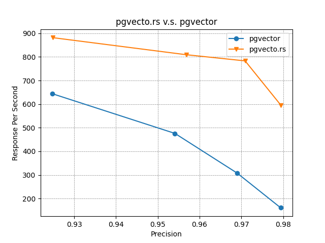
When the vbase mode is enabled, pgvecto.rs can achieve over 2x more responses per second compared to pgvector on various filter probabilities.
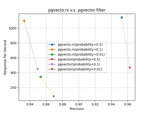
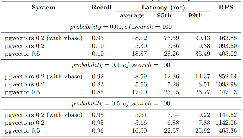
Different quantization methods
pgvecto.rs supports several quantization methods and different low precision indexing. These methods can help to reduce memory usage at different scales. The following figure shows the performance of pgvecto.rs with different quantization methods.
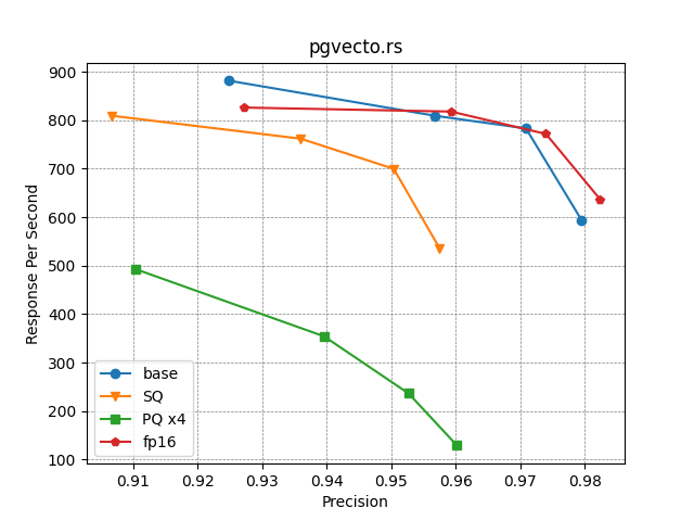
Shortening embeddings (a.k.a Matryoshka Embedding)
OpenAI latest embedding models support shortening embeddings, where developers could simply “remove some numbers from the end of a sequence” and still maintain a valid representation for text.
This enables very flexible usage. For example, when using a vector data store that only supports embeddings up to 1024 dimensions long, developers can now still use our best embedding model text-embedding-3-large and specify a value of 1024 for the dimensions API parameter, which will shorten the embedding down from 3072 dimensions, trading off some accuracy in exchange for the smaller vector size.
These are the performance benchmarks for the shortened embeddings. The dbpedia-entities-openai3-text-embedding-3-large-3072-1M dataset is used for the benchmark. The original embeddings have 3072 dimensions, while the shortened embeddings have dimensions of 256 and 1024. The benchmark was conducted using a VM with specifications of n2-standard-8 (8 vCPUs, 32 GB memory) on Google Cloud.
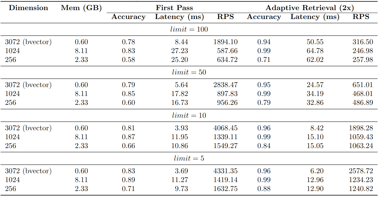
First Pass in the benchmark shows that the accuracy of the shortened embeddings is not as good as the full embeddings. 256D HNSW index only achieves ~65% accuracy, while 1024D HNSW index achieves ~85% accuracy.
However, the accuracy of the shortened embeddings surpasses 95% when adaptive retrieval is employed. Additionally, adopting this approach leads to significant improvements in terms of RPS (Requests Per Second) and latency.
Binary vectors
pgvecto.rs supports binary vectors. The bvector type is optimized for storage and performance. It uses a bit-packed representation to store the binary vector. The distance calculation is also optimized for binary vectors.
Here are some performance benchmarks for the bvector type. We use the dbpedia-entities-openai3-text-embedding-3-large-3072-1M dataset for the benchmark. The VM is n2-standard-8 (8 vCPUs, 32 GB memory) on Google Cloud.
We upsert 1M binary vectors into the table and then run a KNN query for each embedding. It only takes about 600MB memory to index 1M binary vectors, while the vector type takes about 18GB memory to index the same number of vectors.
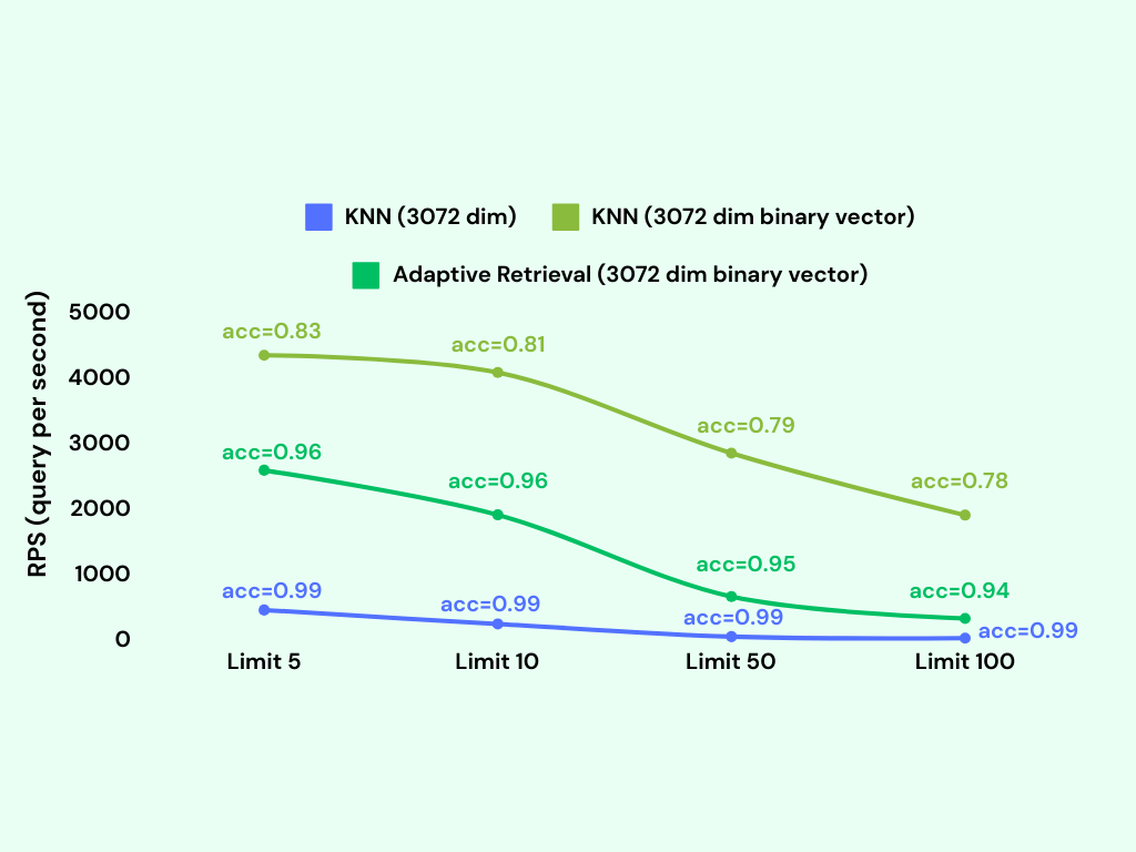
We can see that the bvector’s accuracy is not as good as the vector type, but it exceeds 95% if we adopt adaptive retrieval.
7 - Reference
7.1 - Schema
Here is the schema provided by pgvecto.rs.
List of data types
| Name | Description |
|---|---|
| vector | vector, scalar type of which is binary32 defined in IEEE 754-2008 |
| vecf16 | vector, scalar type of which is binary16 defined in IEEE 754-2008 |
| veci8 | vector, scalar type of which is 8-bit Integer |
| svector | sparse vector, scalar type of which is binary32 defined in IEEE 754-2008 |
| bvector | binary vector, a fixed-length bit string |
| vector_index_stat | a composite type representing vector index statistics |
List of operators
| Name | Left arg type | Right arg type | Result type | Description |
|---|---|---|---|---|
| + | vector | vector | vector | element-wise arithmetic |
| + | vecf16 | vecf16 | vecf16 | element-wise arithmetic |
| + | veci8 | veci8 | veci8 | element-wise arithmetic |
| + | svector | svector | svector | element-wise arithmetic |
| - | vector | vector | vector | element-wise arithmetic |
| - | vecf16 | vecf16 | vecf16 | element-wise arithmetic |
| - | veci8 | veci8 | veci8 | element-wise arithmetic |
| - | svector | svector | svector | element-wise arithmetic |
| & | bvector | bvector | bvector | element-wise logical AND |
| | | bvector | bvector | bvector | element-wise logical OR |
| ^ | bvector | bvector | bvector | element-wise logical XOR |
| = | vector | vector | boolean | dictionary order comparison |
| = | vecf16 | vecf16 | boolean | dictionary order comparison |
| = | veci8 | veci8 | boolean | dictionary order comparison |
| = | svector | svector | boolean | dictionary order comparison |
| = | bvector | bvector | boolean | dictionary order comparison |
| <> | vector | vector | boolean | dictionary order comparison |
| <> | vecf16 | vecf16 | boolean | dictionary order comparison |
| <> | veci8 | veci8 | boolean | dictionary order comparison |
| <> | svector | svector | boolean | dictionary order comparison |
| <> | bvector | bvector | boolean | dictionary order comparison |
| < | vector | vector | boolean | dictionary order comparison |
| < | vecf16 | vecf16 | boolean | dictionary order comparison |
| < | veci8 | veci8 | boolean | dictionary order comparison |
| < | svector | svector | boolean | dictionary order comparison |
| < | bvector | bvector | boolean | dictionary order comparison |
| > | vector | vector | boolean | dictionary order comparison |
| > | vecf16 | vecf16 | boolean | dictionary order comparison |
| > | veci8 | veci8 | boolean | dictionary order comparison |
| > | svector | svector | boolean | dictionary order comparison |
| > | bvector | bvector | boolean | dictionary order comparison |
| <= | vector | vector | boolean | dictionary order comparison |
| <= | vecf16 | vecf16 | boolean | dictionary order comparison |
| <= | veci8 | veci8 | boolean | dictionary order comparison |
| <= | svector | svector | boolean | dictionary order comparison |
| <= | bvector | bvector | boolean | dictionary order comparison |
| >= | vector | vector | boolean | dictionary order comparison |
| >= | vecf16 | vecf16 | boolean | dictionary order comparison |
| >= | veci8 | veci8 | boolean | dictionary order comparison |
| >= | svector | svector | boolean | dictionary order comparison |
| >= | bvector | bvector | boolean | dictionary order comparison |
| <-> | vector | vector | real | squared Euclidean distance |
| <-> | vecf16 | vecf16 | real | squared Euclidean distance |
| <-> | veci8 | veci8 | real | squared Euclidean distance |
| <-> | svector | svector | real | squared Euclidean distance |
| <-> | bvector | bvector | real | squared Euclidean distance |
| <#> | vector | vector | real | negative dot product |
| <#> | vecf16 | vecf16 | real | negative dot product |
| <#> | veci8 | veci8 | real | negative dot product |
| <#> | svector | svector | real | negative dot product |
| <#> | bvector | bvector | real | negative dot product |
| <=> | vector | vector | real | cosine distance |
| <=> | vecf16 | vecf16 | real | cosine distance |
| <=> | veci8 | veci8 | real | cosine distance |
| <=> | svector | svector | real | cosine distance |
| <=> | bvector | bvector | real | cosine distance |
| <~> | bvector | bvector | real | jaccard distance |
List of functions
| Name | Argument type | Result type | Description |
|---|---|---|---|
| pgvectors_upgrade | void | Administration function for upgrading pgvecto.rs. |
|
| to_svector | dims integer, index integer[], value real[] | svector | Construct a sparse vector from two arrays of indexes and values |
| binarize | vector vector | bvector | Binarize a vector. All positive elements are set to 1, otherwise 0. |
| text2vec_openai | input text, model text | vector | Embedding function for OpenAI embeddings API. |
| text2vec_openai_v3 | input text | vector | Embedding function for OpenAI embeddings API. The model is set to text-embedding-3-small. |
List of casts
| Source type | Target type | Implicit? |
|---|---|---|
| real[] | vector | yes |
| vector | real[] | yes |
| vector | vecf16 | no |
| vecf16 | vector | no |
| vector | veci8 | no |
| veci8 | vector | no |
| vector | svector | no |
| svector | vector | no |
| vector | bvector | no |
| bvector | vector | no |
List of access methods
| Name | Type | Description |
|---|---|---|
| vectors | Index | pgvecto.rs vector index |
List of operator families
| AM | Operator family | Applicable types |
|---|---|---|
| vectors | vector_cos_ops | vector |
| vectors | vector_dot_ops | vector |
| vectors | vector_l2_ops | vector |
| vectors | vecf16_cos_ops | vecf16 |
| vectors | vecf16_dot_ops | vecf16 |
| vectors | vecf16_l2_ops | vecf16 |
| vectors | veci8_cos_ops | veci8 |
| vectors | veci8_dot_ops | veci8 |
| vectors | veci8_l2_ops | veci8 |
| vectors | svector_cos_ops | svector |
| vectors | svector_dot_ops | svector |
| vectors | svector_l2_ops | svector |
| vectors | bvector_cos_ops | bvector |
| vectors | bvector_dot_ops | bvector |
| vectors | bvector_l2_ops | bvector |
| vectors | bvector_jaccard_ops | bvector |
List of operator classes
| AM | Input type | Operator class | Default? | Description |
|---|---|---|---|---|
| vectors | vector | vector_l2_ops | no | squared Euclidean distance |
| vectors | vector | vector_dot_ops | no | negative dot product |
| vectors | vector | vector_cos_ops | no | cosine distance |
| vectors | vecf16 | vecf16_l2_ops | no | squared Euclidean distance |
| vectors | vecf16 | vecf16_dot_ops | no | negative dot product |
| vectors | vecf16 | vecf16_cos_ops | no | cosine distance |
| vectors | veci8 | veci8_l2_ops | no | squared Euclidean distance |
| vectors | veci8 | veci8_dot_ops | no | negative dot product |
| vectors | veci8 | veci8_cos_ops | no | cosine distance |
| vectors | svector | svector_l2_ops | no | squared Euclidean distance |
| vectors | svector | svector_dot_ops | no | negative dot product |
| vectors | svector | svector_cos_ops | no | cosine distance |
| vectors | bvector | bvector_l2_ops | no | squared Euclidean distance |
| vectors | bvector | bvector_dot_ops | no | negative dot product |
| vectors | bvector | bvector_cos_ops | no | cosine distance |
| vectors | bvector | bvector_jaccard_ops | no | jaccard distance |
List of views
| Name | Description |
|---|---|
| pg_vector_index_stat | A view provided for vector index statistics |
7.2 - Indexing Options
We utilize TOML syntax to express the index’s configuration. Here’s what each key in the configuration signifies:
| Key | Type | Description |
|---|---|---|
| segment | table | Options for segments. |
| optimizing | table | Options for background optimizing. |
| indexing | table | The algorithm to be used for indexing. |
Options for table segment
| Key | Type | Range | Default | Description |
|---|---|---|---|---|
| max_growing_segment_size | integer | [1, 4_000_000_000] |
20_000 |
Maximum size of unindexed vectors. |
| max_sealed_segment_size | integer | [1, 4_000_000_000] |
1_000_000 |
Maximum size of vectors for indexing. |
Options for table optimizing
| Key | Type | Range | Default | Description |
|---|---|---|---|---|
| optimizing_threads | integer | [1, 65535] |
sqrt of the number of cores | Maximum threads for indexing. |
| sealing_secs | integer | [1, 60] |
60 |
See below. |
| sealing_size | integer | [1, 4_000_000_000] |
1 |
See below. |
If a write segment larger than sealing_size do not accept new data for sealing_secs seconds, the write segment will be turned to a sealed segment.
Options for table indexing
| Key | Type | Description |
|---|---|---|
| flat | table | If this table is set, brute force algorithm will be used for the index. |
| ivf | table | If this table is set, IVF will be used for the index. |
| hnsw | table | If this table is set, HNSW will be used for the index. |
You can choose only one algorithm in above indexing algorithms. Default value is hnsw.
Options for table flat
| Key | Type | Description |
|---|---|---|
| quantization | table | The algorithm to be used for quantization. |
Options for table ivf
| Key | Type | Range | Default | Description |
|---|---|---|---|---|
| nlist | integer | [1, 1_000_000] |
1000 |
Number of cluster units. |
| nsample | integer | [1, 1_000_000] |
65536 |
Number of samples for K-Means clustering. |
| least_iterations | integer | [1, 1_000_000] |
16 |
Least iterations for K-Means clustering. |
| iterations | integer | [1, 1_000_000] |
500 |
Max iterations for K-Means clustering. |
| quantization | table | The quantization algorithm to be used. |
Options for table hnsw
| Key | Type | Range | Default | Description |
|---|---|---|---|---|
| m | integer | [4, 128] |
12 |
Maximum degree of the node. |
| ef_construction | integer | [10, 2000] |
300 |
Search scope in building. |
| quantization | table | The quantization algorithm to be used. |
Options for table quantization
| Key | Type | Description |
|---|---|---|
| trivial | table | If this table is set, no quantization is used. |
| scalar | table | If this table is set, scalar quantization is used. |
| product | table | If this table is set, product quantization is used. |
You can choose only one algorithm in above indexing algorithms. Default value is trivial.
Options for table product
| Key | Type | Range | Default | Description |
|---|---|---|---|---|
| sample | integer | [1, 1_000_000] |
65535 |
Samples to be used for quantization. |
| ratio | enum | "x4", "x8", "x16", "x32", "x64" |
"x4" |
Compression ratio for quantization. |
Compression ratio is how many memory you are saved for saving vectors. For example, "x4" is compared to before. If you are creating indexes on vecf16, "x4" is compared to before.
7.3 - Search Options
Search options are specified by PostgreSQL GUC.
Options for ivf
These options only work for IVF algorithm. Refer to Indexing.
| Option | Type | Range | Default | Description |
|---|---|---|---|---|
| vectors.ivf_nprobe | integer | [1, 1_000_000] |
10 |
Number of lists to scan. |
Options for hnsw
These options only work for HNSW algorithm. Refer to Indexing.
| Option | Type | Range | Default | Description |
|---|---|---|---|---|
| vectors.hnsw_ef_search | integer | [1, 65535] |
100 |
Search scope of HNSW. |
Other Options
Query options for search mode: .
| Option | Type | Range | Default | Description |
|---|---|---|---|---|
| vectors.search_mode | enum | "basic", "vbase" |
"vbase" |
Search mode, Refer to Search |
| vectors.pgvector_compatibility | boolean | off |
Enable or disable pgvector compatibility, Refer to pgvector compatibility |
|
| vectors.enable_index | boolean | on |
Enable or disable the query planner’s use of vector types. |
7.4 - Vector Types
In the previous sections Indexing and Search, we encountered the vector type. This section will explore additional vector types and their applications in the realm of vector search.
- Half-Precision Vector
- 8-Bit Integer Vector since v0.3.0
- Sparse Vector since v0.3.0
- Binary Vector since v0.3.0
Low-precision Indexing
since v0.3.0To improve the speed of queries on the vector column, consider creating a low-precision index using vecf16, veci8, or bvector types instead of a vector type.
Shortening Embedding
since v0.3.0Certain embedding models like OpenAI text-embedding-3-small support shortening embeddings, which involves removing some numbers from the end of the sequence without losing the embedding’s concept-representing properties.
In some cases, it may be necessary to change the embedding dimension after generation. The pgvecto.rs offers an approach to query by shortened embeddings.
Shortened embeddings are supported by all data types in pgvecto.rs since version v0.3.0.
Casts
This diagram shows the conversion between different data types, where the types connected by arrows can be cast to each other:
Among them, ARRAY is a native type of postgreSQL, others are types defined by pgvecto.rs.
Here are some examples of vector type casting:
7.4.1 - Half-Precision Vector: `vecf16`
Stored as a half-precision number format, vecf16 takes advantage of the 16-bit float, which uses half the memory and bandwidth compared to vector.
Here’s an example of creating a table with a vecf16 column and inserting values:
Index can be created on vecf16 type as well.
We support three operators to calculate the distance between two vecf16 values.
<->(vecf16_l2_ops): squared Euclidean distance, defined as .<#>(vecf16_dot_ops): negative dot product, defined as .<=>(vecf16_cos_ops): cosine distance, defined as .
7.4.2 - 8-Bit Integer Vector: `veci8`
Int8 is a data type used to represent signed integers. It stands for “integer 8-bit” and typically uses 8 bits of memory to store a value. This allows it to represent integer values ranging from -128 to 127.
Since each element in the vector only requires 8 bits (1 byte) of memory, veci8 can help reduce the overall memory footprint of your program.
Here’s an example of creating a table with a veci8 column and inserting values:
Index can be created on veci8 type as well.
We support three operators to calculate the distance between two veci8 values.
<->(veci8_l2_ops): squared Euclidean distance, defined as .<#>(veci8_dot_ops): negative dot product, defined as .<=>(veci8_cos_ops): cosine distance, defined as .
7.4.3 - Sparse Vector: `svector`
Unlike dense vectors, sparse vectors are very high-dimensional but contain few non-zero values.
Typically, sparse vectors can be created from:
- Word co-occurrence matrices
- Term frequency-inverse document frequency (TF-IDF) vectors
- User-item interaction matrices
- Network adjacency matrices
Sparse vectors in pgvecto.rs are called svector.
Here’s an example of creating a table with a svector column and inserting values:
Index can be created on svector type as well.
We support three operators to calculate the distance between two svector values.
<->(svector_l2_ops): squared Euclidean distance, defined as .<#>(svector_dot_ops): negative dot product, defined as .<=>(svector_cos_ops): cosine distance, defined as .
There is also a function to_svector to create a svector. It will set the value at the specified position.
7.4.4 - Binary Vector: `bvector`
The bvector type is a binary vector type in pgvecto.rs. It represents a binary vector, which is a vector where each component can take on two possible values, typically 0 and 1.
Here’s an example of creating a table with a bvector column and inserting values:
Index can be created on bvector type as well.
We support three operators to calculate the distance between two bvector values.
<->(bvector_l2_ops): squared Euclidean distance, defined as . The Hamming distance is equivalent to the squared Euclidean distance for binary vectors.<#>(bvector_dot_ops): negative dot product, defined as .<=>(bvector_cos_ops): cosine distance, defined as .<~>(bvector_jaccard_ops): Jaccard distance, defined as .
There is also a function binarize to build bvector from vector. It truncates vector elements to integers of 0 or 1.
Performance
The bvector type is optimized for storage and performance. It uses a bit-packed representation to store the binary vector. The distance calculation is also optimized for binary vectors.
Here are some performance benchmarks for the bvector type. We use the dbpedia-entities-openai3-text-embedding-3-large-3072-1M dataset for the benchmark. The VM is n2-standard-8 (8 vCPUs, 32 GB memory) on Google Cloud.
We upsert 1M binary vectors into the table and then run a KNN query for each embedding. It only takes about 600MB memory to index 1M binary vectors, while the vector type takes about 18GB memory to index the same number of vectors.
We can see that the bvector’s accuracy is not as good as the vector type, but it exceeds 95% if we adopt adaptive retrieval.
8 - Community
8.1 - Contributing to `pgvecto.rs`
We welcome all kinds of contributions from the open-source community, individuals, and partners. If you’re interested in contributing, hopefully, this document makes the process for contributing clear.
Contributors and people new to open source alike will find the following guides especially useful:
Code of conduct
A code of conduct is a document that establishes expectations for behavior for the project’s participants. Adopting, and enforcing, a code of conduct can help create a positive social atmosphere for the community.
If you do not know what code of conduct is, please have a look at Your Code of Conduct | Open Source Guides.
Get involved
Our community is always looking for enthusiasts to help in all different ways.
⚽ Simply start using pgvecto.rs
Go through the Getting Started guide. Does everything work as expected? If not, we’re always looking for improvements. Chat with us on 💬 Discord or file an issue on GitHub.
🙋 Triaging Issues and Pull Requests
One great way you can contribute to the project without writing any code is to help triage issues and pull requests as they come in.
- Ask for more information if you believe the issue does not provide all the details required to solve it.
- Suggest labels that can help categorize issues.
- Flag issues that are stale or that should be closed.
- Ask for test plans and review code.
👨💻 Contribute to pgvecto.rs
If you find an issue you would like to fix, open a pull request. Please read development tutorials to get started.
👉 Improve documentation
Everyone loves documentation. If you find anything that is confusing or can be improved, you can click “Edit this page” at the bottom of most docs, which takes you to the GitHub interface to make and propose changes.
💬 Discuss pgvecto.rs on Discord
Chat with us on 💬 Discord.
8.2 - Roadmap
We strongly suggest you explore our new VectorChord implementation, offering enhanced stability and performance. Users are advised to transition to VectorChord. Refer to the migration guide for assistance.
Midterm Plan
Sparse Vector Support
Sparse vectors have shown excellent performance in tasks such as RAG and text retrieval, and can improve the results of dense vectors. Therefore, we plan to support sparse vector indexing.
Better support for streaming workloads
As a database, it is important to support flexible insertion and deletion of vector data. However, the current mainstream algorithm HNSW does not have good support for deletion because it requires rebuilding the index. Therefore, we plan to follow the DiskANN article and support the Vamana algorithm. The Vamana algorithm is an incremental indexing algorithm based on Graph that can support deletion and insertion of vectors without rebuilding the index.
More vectors on a single machine
Supporting more vectors under the same resources is very important for users to save costs. Currently, we have supported users to store vectors in fp16 format, which requires only half of the memory and space with little loss of accuracy. We also plan to support more vector formats, such as fp8 and int8, to further reduce storage and memory consumption. At the same time, we are also exploring SSD-based vector indexing algorithms such as DiskANN.
Physical and Streaming Replication
pgvecto.rs is currently an independent storage system separate from PostgreSQL, managing index memory and storage on its own. Therefore it doesn’t support physical replication out of the box. We plan to implement a custom WAL resource manager to meet the requirements of physical replication and make it easier for users to use replication in PG.
Longterm plan
1B vectors inside PostgreSQL
Our ultimate goal is to support 1 billion vectors in PostgreSQL. However, there are many challenges that need to be overcome to reach this goal. It may be necessary to implement a custom vector storage solution using the table access method, or to use a distributed shard such as Citus. We have not yet explored this area extensively, so interested developers are encouraged to discuss it with us.
Talk with us
Want to jump in? Welcome discussions and contributions!
- Chat with us on 💬 Discord
- Have a look at
good first issue 💖issues! - More on contributing page
These items are not essential for an MVP, but are a part of our longer term plans. Feel free to jump in on these if you’re interested!
To be added in the future.
8.3 - Adopters
- immich is a self-hosted photo and video backup solution directly from your mobile phone. it is using pgvecto.rs to search.
- postgresql_embedded is a set of utilities for installing, running and managing PostgreSQL and extensions in Rust with support for installing pgvecto.rs.
Add your app here
If you are using pgvecto.rs in your app, please edit this page. We are glad to get your feedback and help you to improve your experience with pgvecto.rs.
9 - Developers
9.1 - Development
Set up development environment
You can set up development environment simply using envd. It will create a docker container and install all the dependencies for you.
Or you can setup development environment following these steps manually:
- Install base dependency.
- Install
clang-16. Other versions ofclangare not supported.
- Install Rust. Do not install
rustcusing a package manager.
- Clone the Repository.
- Install
cargo-pgrx.
cargo-pgrx is a helpful tool to develop a PostgreSQL extension. You can read the document in https://docs.rs/crate/cargo-pgrx/latest.
Cross compilation
Assuming that you build binary and schema for aarch64 target in x86_64 host environment, you can follow these steps:
- Install cross compilation toolchain.
Set environment variables.
Set emulator, linker and sysroot for Rust by adding the following section to the end of ~/.cargo/config.toml.
- Generate PostgreSQL header files on target architecture. It can be done with
cargo-pgrxand you can also take advantages of files undervendor/pgrx_configandvendor/pgrx_binding. For details, please refer to the documentation ofpgrx.
Debug
Debug information included in the compiled binary even in release mode so you can always use gdb for debugging.
For a debug build, backtrace is printed when a thread in background worker process panics, but not for a session process error. For a release build, backtrace is never printed. But if you set environment variable RUST_BACKTRACE to 1, all backtraces are printed. It’s recommended for you to debug a release build with the command RUST_BACKTRACE=1 cargo pgrx run --release.